


Big Data Analytics - Data Visualization
In order to understand data, it is often useful to visualize it. Normally in Big Data applications, the interest relies in finding insight rather than just making beautiful plots. The following are examples of different approaches to understanding data using plots.
To start analyzing the flights data, we can start by checking if there are correlations between numeric variables. This code is also available in bda/part1/data_visualization/data_visualization.R file.
# Install the package corrplot by running
install.packages('corrplot')

# then load the library
library(corrplot)

# Load the following libraries
library(nycflights13)
library(ggplot2)
library(data.table)
library(reshape2)

# We will continue working with the flights data
DT <- as.data.table(flights)
head(DT) # take a look

# We select the numeric variables after inspecting the first rows.
numeric_variables = c('dep_time', 'dep_delay',
   'arr_time', 'arr_delay', 'air_time', 'distance')

# Select numeric variables from the DT data.table
dt_num = DT[, numeric_variables, with = FALSE]

# Compute the correlation matrix of dt_num
cor_mat = cor(dt_num, use = "complete.obs")

print(cor_mat)
### Here is the correlation matrix
#              dep_time   dep_delay   arr_time   arr_delay    air_time    distance
# dep_time   1.00000000  0.25961272 0.66250900  0.23230573 -0.01461948 -0.01413373
# dep_delay  0.25961272  1.00000000 0.02942101  0.91480276 -0.02240508 -0.02168090
# arr_time   0.66250900  0.02942101 1.00000000  0.02448214  0.05429603  0.04718917
# arr_delay  0.23230573  0.91480276 0.02448214  1.00000000 -0.03529709 -0.06186776
# air_time  -0.01461948 -0.02240508 0.05429603 -0.03529709  1.00000000  0.99064965
# distance  -0.01413373 -0.02168090 0.04718917 -0.06186776  0.99064965  1.00000000

# We can display it visually to get a better understanding of the data
corrplot.mixed(cor_mat, lower = "circle", upper = "ellipse")

# save it to disk
png('corrplot.png')
print(corrplot.mixed(cor_mat, lower = "circle", upper = "ellipse"))
dev.off()
This code generates the following correlation matrix visualization −
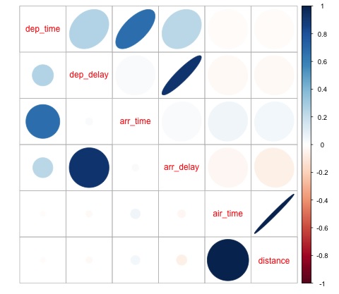
We can see in the plot that there is a strong correlation between some of the variables in the dataset. For example, arrival delay and departure delay seem to be highly correlated. We can see this because the ellipse shows an almost lineal relationship between both variables, however, it is not simple to find causation from this result.
We can’t say that as two variables are correlated, that one has an effect on the other. Also we find in the plot a strong correlation between air time and distance, which is fairly reasonable to expect as with more distance, the flight time should grow.
We can also do univariate analysis of the data. A simple and effective way to visualize distributions are box-plots. The following code demonstrates how to produce box-plots and trellis charts using the ggplot2 library. This code is also available in bda/part1/data_visualization/boxplots.R file.
source('data_visualization.R')
### Analyzing Distributions using box-plots
# The following shows the distance as a function of the carrier

p = ggplot(DT, aes(x = carrier, y = distance, fill = carrier)) + # Define the carrier
   in the x axis and distance in the y axis
   geom_box-plot() + # Use the box-plot geom
   theme_bw() + # Leave a white background - More in line with tufte's
      principles than the default
   guides(fill = FALSE) + # Remove legend
   labs(list(title = 'Distance as a function of carrier', # Add labels
      x = 'Carrier', y = 'Distance'))
p
# Save to disk
png(‘boxplot_carrier.png’)
print(p)
dev.off()

# Let's add now another variable, the month of each flight
# We will be using facet_wrap for this
p = ggplot(DT, aes(carrier, distance, fill = carrier)) +
   geom_box-plot() +
   theme_bw() +
   guides(fill = FALSE) +
   facet_wrap(~month) + # This creates the trellis plot with the by month variable
   labs(list(title = 'Distance as a function of carrier by month',
      x = 'Carrier', y = 'Distance'))
p
# The plot shows there aren't clear differences between distance in different months

# Save to disk
png('boxplot_carrier_by_month.png')
print(p)
dev.off()
Big Data Analytics - Introduction to R
This section is devoted to introduce the users to the R programming language. R can be downloaded from the cran website. For Windows users, it is useful to install rtools and the rstudio IDE.
The general concept behind R is to serve as an interface to other software developed in compiled languages such as C, C++, and Fortran and to give the user an interactive tool to analyze data.
Navigate to the folder of the book zip file bda/part2/R_introduction and open the R_introduction.Rproj file. This will open an RStudio session. Then open the 01_vectors.R file. Run the script line by line and follow the comments in the code. Another useful option in order to learn is to just type the code, this will help you get used to R syntax. In R comments are written with the # symbol.
In order to display the results of running R code in the book, after code is evaluated, the results R returns are commented. This way, you can copy paste the code in the book and try directly sections of it in R.
# Create a vector of numbers
numbers = c(1, 2, 3, 4, 5)
print(numbers)

# [1] 1 2 3 4 5
# Create a vector of letters
ltrs = c('a', 'b', 'c', 'd', 'e')
# [1] "a" "b" "c" "d" "e"

# Concatenate both
mixed_vec = c(numbers, ltrs)
print(mixed_vec)
# [1] "1" "2" "3" "4" "5" "a" "b" "c" "d" "e"
Let’s analyze what happened in the previous code. We can see it is possible to create vectors with numbers and with letters. We did not need to tell R what type of data type we wanted beforehand. Finally, we were able to create a vector with both numbers and letters. The vector mixed_vec has coerced the numbers to character, we can see this by visualizing how the values are printed inside quotes.
The following code shows the data type of different vectors as returned by the function class. It is common to use the class function to "interrogate" an object, asking him what his class is.
### Evaluate the data types using class

### One dimensional objects
# Integer vector
num = 1:10
class(num)
# [1] "integer"

# Numeric vector, it has a float, 10.5
num = c(1:10, 10.5)
class(num)
# [1] "numeric"

# Character vector
ltrs = letters[1:10]
class(ltrs)
# [1] "character"

# Factor vector
fac = as.factor(ltrs)
class(fac)
# [1] "factor"
R supports two-dimensional objects also. In the following code, there are examples of the two most popular data structures used in R: the matrix and data.frame.
# Matrix
M = matrix(1:12, ncol = 4)
#      [,1] [,2] [,3] [,4]
# [1,]    1    4    7   10
# [2,]    2    5    8   11
# [3,]    3    6    9   12
lM = matrix(letters[1:12], ncol = 4)
#     [,1] [,2] [,3] [,4]
# [1,] "a"  "d"  "g"  "j"
# [2,] "b"  "e"  "h"  "k"
# [3,] "c"  "f"  "i"  "l"

# Coerces the numbers to character
# cbind concatenates two matrices (or vectors) in one matrix
cbind(M, lM)
#     [,1] [,2] [,3] [,4] [,5] [,6] [,7] [,8]
# [1,] "1"  "4"  "7"  "10" "a"  "d"  "g"  "j"
# [2,] "2"  "5"  "8"  "11" "b"  "e"  "h"  "k"
# [3,] "3"  "6"  "9"  "12" "c"  "f"  "i"  "l"

class(M)
# [1] "matrix"
class(lM)
# [1] "matrix"

# data.frame
# One of the main objects of R, handles different data types in the same object.
# It is possible to have numeric, character and factor vectors in the same data.frame

df = data.frame(n = 1:5, l = letters[1:5])
df
#   n l
# 1 1 a
# 2 2 b
# 3 3 c
# 4 4 d
# 5 5 e
As demonstrated in the previous example, it is possible to use different data types in the same object. In general, this is how data is presented in databases, APIs part of the data is text or character vectors and other numeric. In is the analyst job to determine which statistical data type to assign and then use the correct R data type for it. In statistics we normally consider variables are of the following types −
- Numeric
- Nominal or categorical
- Ordinal
In R, a vector can be of the following classes −
- Numeric - Integer
- Factor
- Ordered Factor
R provides a data type for each statistical type of variable. The ordered factor is however rarely used, but can be created by the function factor, or ordered.
The following section treats the concept of indexing. This is a quite common operation, and deals with the problem of selecting sections of an object and making transformations to them.
# Let's create a data.frame
df = data.frame(numbers = 1:26, letters)
head(df)
#      numbers  letters
# 1       1       a
# 2       2       b
# 3       3       c
# 4       4       d
# 5       5       e
# 6       6       f

# str gives the structure of a data.frame, it’s a good summary to inspect an object
str(df)
#   'data.frame': 26 obs. of  2 variables:
#   $ numbers: int  1 2 3 4 5 6 7 8 9 10 ...
#   $ letters: Factor w/ 26 levels "a","b","c","d",..: 1 2 3 4 5 6 7 8 9 10 ...

# The latter shows the letters character vector was coerced as a factor.
# This can be explained by the stringsAsFactors = TRUE argumnet in data.frame
# read ?data.frame for more information

class(df)
# [1] "data.frame"

### Indexing
# Get the first row
df[1, ]
#     numbers  letters
# 1       1       a

# Used for programming normally - returns the output as a list
df[1, , drop = TRUE]
# $numbers
# [1] 1
#
# $letters
# [1] a
# Levels: a b c d e f g h i j k l m n o p q r s t u v w x y z

# Get several rows of the data.frame
df[5:7, ]
#      numbers  letters
# 5       5       e
# 6       6       f
# 7       7       g

### Add one column that mixes the numeric column with the factor column
df$mixed = paste(df$numbers, df$letters, sep = ’’)

str(df)
# 'data.frame': 26 obs. of  3 variables:
# $ numbers: int  1 2 3 4 5 6 7 8 9 10 ...
# $ letters: Factor w/ 26 levels "a","b","c","d",..: 1 2 3 4 5 6 7 8 9 10 ...
# $ mixed  : chr  "1a" "2b" "3c" "4d" ...

### Get columns
# Get the first column
df[, 1]
# It returns a one dimensional vector with that column

# Get two columns
df2 = df[, 1:2]
head(df2)

#      numbers  letters
# 1       1       a
# 2       2       b
# 3       3       c
# 4       4       d
# 5       5       e
# 6       6       f

# Get the first and third columns
df3 = df[, c(1, 3)]
df3[1:3, ]

#      numbers  mixed
# 1       1     1a
# 2       2     2b
# 3       3     3c

### Index columns from their names
names(df)
# [1] "numbers" "letters" "mixed"
# This is the best practice in programming, as many times indeces change, but
variable names don’t
# We create a variable with the names we want to subset
keep_vars = c("numbers", "mixed")
df4 = df[, keep_vars]

head(df4)
#      numbers  mixed
# 1       1     1a
# 2       2     2b
# 3       3     3c
# 4       4     4d
# 5       5     5e
# 6       6     6f

### subset rows and columns
# Keep the first five rows
df5 = df[1:5, keep_vars]
df5

#      numbers  mixed
# 1       1     1a
# 2       2     2b
# 3       3     3c
# 4       4     4d
# 5       5     5e

# subset rows using a logical condition
df6 = df[df$numbers < 10, keep_vars]
df6

#      numbers  mixed
# 1       1     1a
# 2       2     2b
# 3       3     3c
# 4       4     4d
# 5       5     5e
# 6       6     6f
# 7       7     7g
# 8       8     8h
# 9       9     9i
Big Data Analytics - Introduction to SQL
SQL stands for structured query language. It is one of the most widely used languages for extracting data from databases in traditional data warehouses and big data technologies. In order to demonstrate the basics of SQL we will be working with examples. In order to focus on the language itself, we will be using SQL inside R. In terms of writing SQL code this is exactly as would be done in a database.
The core of SQL are three statements: SELECT, FROM and WHERE. The following examples make use of the most common use cases of SQL. Navigate to the folder bda/part2/SQL_introduction and open the SQL_introduction.Rproj file. Then open the 01_select.R script. In order to write SQL code in R we need to install the sqldf package as demonstrated in the following code.
# Install the sqldf package
install.packages('sqldf')

# load the library
library('sqldf')
library(nycflights13)

# We will be working with the fligths dataset in order to introduce SQL

# Let’s take a look at the table
str(flights)
# Classes 'tbl_d', 'tbl' and 'data.frame': 336776 obs. of  16 variables:

# $ year     : int  2013 2013 2013 2013 2013 2013 2013 2013 2013 2013 ...
# $ month    : int  1 1 1 1 1 1 1 1 1 1 ...
# $ day      : int  1 1 1 1 1 1 1 1 1 1 ...
# $ dep_time : int  517 533 542 544 554 554 555 557 557 558 ...
# $ dep_delay: num  2 4 2 -1 -6 -4 -5 -3 -3 -2 ...
# $ arr_time : int  830 850 923 1004 812 740 913 709 838 753 ...
# $ arr_delay: num  11 20 33 -18 -25 12 19 -14 -8 8 ...
# $ carrier  : chr  "UA" "UA" "AA" "B6" ...

# $ tailnum  : chr  "N14228" "N24211" "N619AA" "N804JB" ...
# $ flight   : int  1545 1714 1141 725 461 1696 507 5708 79 301 ...
# $ origin   : chr  "EWR" "LGA" "JFK" "JFK" ...
# $ dest     : chr  "IAH" "IAH" "MIA" "BQN" ...
# $ air_time : num  227 227 160 183 116 150 158 53 140 138 ...
# $ distance : num  1400 1416 1089 1576 762 ...
# $ hour     : num  5 5 5 5 5 5 5 5 5 5 ...
# $ minute   : num  17 33 42 44 54 54 55 57 57 58 ...
The select statement is used to retrieve columns from tables and do calculations on them. The simplest SELECT statement is demonstrated in ej1. We can also create new variables as shown in ej2.
### SELECT statement
ej1 = sqldf("
   SELECT
   dep_time
   ,dep_delay
   ,arr_time
   ,carrier
   ,tailnum
   FROM
   flights
")

head(ej1)
#    dep_time   dep_delay  arr_time  carrier  tailnum
# 1      517         2      830      UA       N14228
# 2      533         4      850      UA       N24211
# 3      542         2      923      AA       N619AA
# 4      544        -1     1004      B6       N804JB
# 5      554        -6      812      DL       N668DN
# 6      554        -4      740      UA       N39463

# In R we can use SQL with the sqldf function. It works exactly the same as in
a database

# The data.frame (in this case flights) represents the table we are querying
and goes in the FROM statement
# We can also compute new variables in the select statement using the syntax:

# old_variables as new_variable
ej2 = sqldf("
   SELECT
   arr_delay - dep_delay as gain,
   carrier
   FROM
   flights
")

ej2[1:5, ]
#    gain   carrier
# 1    9      UA
# 2   16      UA
# 3   31      AA
# 4  -17      B6
# 5  -19      DL
One of the most common used features of SQL is the group by statement. This allows to compute a numeric value for different groups of another variable. Open the script 02_group_by.R.
### GROUP BY

# Computing the average
ej3 = sqldf("
  SELECT
   avg(arr_delay) as mean_arr_delay,
   avg(dep_delay) as mean_dep_delay,
   carrier
   FROM
   flights
   GROUP BY
   carrier
")

#    mean_arr_delay   mean_dep_delay carrier
# 1       7.3796692      16.725769      9E
# 2       0.3642909       8.586016      AA
# 3      -9.9308886       5.804775      AS
# 4       9.4579733      13.022522      B6
# 5       1.6443409       9.264505      DL
# 6      15.7964311      19.955390      EV
# 7      21.9207048      20.215543      F9
# 8      20.1159055      18.726075      FL
# 9      -6.9152047       4.900585      HA
# 10     10.7747334      10.552041      MQ
# 11     11.9310345      12.586207      OO
# 12      3.5580111      12.106073      UA
# 13      2.1295951       3.782418      US
# 14      1.7644644      12.869421      VX
# 15      9.6491199      17.711744      WN
# 16     15.5569853      18.996330      YV

# Other aggregations
ej4 = sqldf("
   SELECT
   avg(arr_delay) as mean_arr_delay,
   min(dep_delay) as min_dep_delay,
   max(dep_delay) as max_dep_delay,
   carrier
   FROM
   flights
   GROUP BY
   carrier
")

# We can compute the minimun, mean, and maximum values of a numeric value
ej4
#      mean_arr_delay    min_dep_delay   max_dep_delay   carrier
# 1       7.3796692           -24           747          9E
# 2       0.3642909           -24          1014          AA
# 3      -9.9308886           -21           225          AS
# 4       9.4579733           -43           502          B6
# 5       1.6443409           -33           960         DL
# 6      15.7964311           -32           548         EV
# 7      21.9207048           -27           853         F9
# 8      20.1159055           -22           602         FL
# 9      -6.9152047           -16          1301         HA
# 10     10.7747334           -26          1137         MQ
# 11     11.9310345           -14           154         OO
# 12      3.5580111           -20           483         UA
# 13      2.1295951           -19           500         US
# 14      1.7644644           -20           653         VX
# 15      9.6491199           -13           471         WN
# 16     15.5569853           -16           387         YV

### We could be also interested in knowing how many observations each carrier has
ej5 = sqldf("
   SELECT
   carrier, count(*) as count
   FROM
   flights
   GROUP BY
   carrier
")

ej5
#      carrier  count
# 1       9E    18460
# 2       AA   32729
# 3       AS   714
# 4       B6   54635
# 5       DL   48110
# 6       EV   54173
# 7       F9   685
# 8       FL   3260
# 9       HA   342
# 10      MQ   26397
# 11      OO   32
# 12      UA   58665
# 13      US   20536
# 14      VX   5162
# 15      WN   12275
# 16      YV   601
The most useful feature of SQL are joins. A join means that we want to combine table A and table B in one table using one column to match the values of both tables. There are different types of joins, in practical terms, to get started these will be the most useful ones: inner join and left outer join.
# Let’s create two tables: A and B to demonstrate joins.
A = data.frame(c1 = 1:4, c2 = letters[1:4])
B = data.frame(c1 = c(2,4,5,6), c2 = letters[c(2:5)])

A
# c1 c2
# 1  a
# 2  b
# 3  c
# 4  d

B
# c1 c2
# 2  b
# 4  c
# 5  d
# 6  e

### INNER JOIN
# This means to match the observations of the column we would join the tables by.
inner = sqldf("
   SELECT
   A.c1, B.c2
   FROM
   A INNER JOIN B
   ON A.c1 = B.c1
")

# Only the rows that match c1 in both A and B are returned
inner
# c1 c2
#  2  b
#  4  c

### LEFT OUTER JOIN
# the left outer join, sometimes just called left join will return the
# first all the values of the column used from the A table
left = sqldf("
  SELECT
   A.c1, B.c2
  FROM
   A LEFT OUTER JOIN B
   ON A.c1 = B.c1
")

# Only the rows that match c1 in both A and B are returned
left
#   c1    c2
#    1  <NA>
#    2    b
#    3  <NA>
#    4    c


