Big Data Analytics - Data Analyst
A data analyst has reporting-oriented profile, having experience in extracting and analyzing data from traditional data warehouses using SQL. Their tasks are normally either on the side of data storage or in reporting general business results. Data warehousing is by no means simple, it is just different to what a data scientist does.
Many organizations struggle hard to find competent data scientists in the market. It is however a good idea to select prospective data analysts and teach them the relevant skills to become a data scientist. This is by no means a trivial task and would normally involve the person doing a master degree in a quantitative field, but it is definitely a viable option. The basic skills a competent data analyst must have are listed below −
- Business understanding
- SQL programming
- Report design and implementation
- Dashboard development
Big Data Analytics - Data Scientist
The role of a data scientist is normally associated with tasks such as predictive modeling, developing segmentation algorithms, recommender systems, A/B testing frameworks and often working with raw unstructured data.
The nature of their work demands a deep understanding of mathematics, applied statistics and programming. There are a few skills common between a data analyst and a data scientist, for example, the ability to query databases. Both analyze data, but the decision of a data scientist can have a greater impact in an organization.
Here is a set of skills a data scientist normally need to have −
- Programming in a statistical package such as: R, Python, SAS, SPSS, or Julia
- Able to clean, extract, and explore data from different sources
- Research, design, and implementation of statistical models
- Deep statistical, mathematical, and computer science knowledge
In big data analytics, people normally confuse the role of a data scientist with that of a data architect. In reality, the difference is quite simple. A data architect defines the tools and the architecture the data would be stored at, whereas a data scientist uses this architecture. Of course, a data scientist should be able to set up new tools if needed for ad-hoc projects, but the infrastructure definition and design should not be a part of his task.
Big Data Analytics - Problem Definition
Through this tutorial, we will develop a project. Each subsequent chapter in this tutorial deals with a part of the larger project in the mini-project section. This is thought to be an applied tutorial section that will provide exposure to a real-world problem. In this case, we would start with the problem definition of the project.
Project Description
The objective of this project would be to develop a machine learning model to predict the hourly salary of people using their curriculum vitae (CV) text as input.
Using the framework defined above, it is simple to define the problem. We can define X = {x1, x2, …, xn} as the CV’s of users, where each feature can be, in the simplest way possible, the amount of times this word appears. Then the response is real valued, we are trying to predict the hourly salary of individuals in dollars.
These two considerations are enough to conclude that the problem presented can be solved with a supervised regression algorithm.
Problem Definition
Problem Definition is probably one of the most complex and heavily neglected stages in the big data analytics pipeline. In order to define the problem a data product would solve, experience is mandatory. Most data scientist aspirants have little or no experience in this stage.
Most big data problems can be categorized in the following ways −
- Supervised classification
- Supervised regression
- Unsupervised learning
- Learning to rank
Let us now learn more about these four concepts.
Supervised Classification
Given a matrix of features X = {x1, x2, ..., xn} we develop a model M to predict different classes defined as y = {c1, c2, ..., cn}. For example: Given transactional data of customers in an insurance company, it is possible to develop a model that will predict if a client would churn or not. The latter is a binary classification problem, where there are two classes or target variables: churn and not churn.
Other problems involve predicting more than one class, we could be interested in doing digit recognition, therefore the response vector would be defined as: y = {0, 1, 2, 3, 4, 5, 6, 7, 8, 9}, a-state-of-the-art model would be convolutional neural network and the matrix of features would be defined as the pixels of the image.
Supervised Regression
In this case, the problem definition is rather similar to the previous example; the difference relies on the response. In a regression problem, the response y ∈ ℜ, this means the response is real valued. For example, we can develop a model to predict the hourly salary of individuals given the corpus of their CV.
Unsupervised Learning
Management is often thirsty for new insights. Segmentation models can provide this insight in order for the marketing department to develop products for different segments. A good approach for developing a segmentation model, rather than thinking of algorithms, is to select features that are relevant to the segmentation that is desired.
For example, in a telecommunications company, it is interesting to segment clients by their cellphone usage. This would involve disregarding features that have nothing to do with the segmentation objective and including only those that do. In this case, this would be selecting features as the number of SMS used in a month, the number of inbound and outbound minutes, etc.
Learning to Rank
This problem can be considered as a regression problem, but it has particular characteristics and deserves a separate treatment. The problem involves given a collection of documents we seek to find the most relevant ordering given a query. In order to develop a supervised learning algorithm, it is needed to label how relevant an ordering is, given a query.
It is relevant to note that in order to develop a supervised learning algorithm, it is needed to label the training data. This means that in order to train a model that will, for example, recognize digits from an image, we need to label a significant amount of examples by hand. There are web services that can speed up this process and are commonly used for this task such as amazon mechanical turk. It is proven that learning algorithms improve their performance when provided with more data, so labeling a decent amount of examples is practically mandatory in supervised learning.
Big Data Analytics - Data Collection
Data collection plays the most important role in the Big Data cycle. The Internet provides almost unlimited sources of data for a variety of topics. The importance of this area depends on the type of business, but traditional industries can acquire a diverse source of external data and combine those with their transactional data.
For example, let’s assume we would like to build a system that recommends restaurants. The first step would be to gather data, in this case, reviews of restaurants from different websites and store them in a database. As we are interested in raw text, and would use that for analytics, it is not that relevant where the data for developing the model would be stored. This may sound contradictory with the big data main technologies, but in order to implement a big data application, we simply need to make it work in real time.
Twitter Mini Project
Once the problem is defined, the following stage is to collect the data. The following miniproject idea is to work on collecting data from the web and structuring it to be used in a machine learning model. We will collect some tweets from the twitter rest API using the R programming language.
First of all create a twitter account, and then follow the instructions in the twitteR package vignette to create a twitter developer account. This is a summary of those instructions −
- Go to https://twitter.com/apps/new and log in.
- After filling in the basic info, go to the "Settings" tab and select "Read, Write and Access direct messages".
- Make sure to click on the save button after doing this
- In the "Details" tab, take note of your consumer key and consumer secret
- In your R session, you’ll be using the API key and API secret values
- Finally run the following script. This will install the twitteR package from its repository on github.
install.packages(c("devtools", "rjson", "bit64", "httr"))

# Make sure to restart your R session at this point
library(devtools)
install_github("geoffjentry/twitteR")
We are interested in getting data where the string "big mac" is included and finding out which topics stand out about this. In order to do this, the first step is collecting the data from twitter. Below is our R script to collect required data from twitter. This code is also available in bda/part1/collect_data/collect_data_twitter.R file.
rm(list = ls(all = TRUE)); gc() # Clears the global environment
library(twitteR)
Sys.setlocale(category = "LC_ALL", locale = "C")

### Replace the xxx’s with the values you got from the previous instructions

# consumer_key = "xxxxxxxxxxxxxxxxxxxx"
# consumer_secret = "xxxxxxxxxxxxxxxxxxxxxxxxxxxxxxxxxxxxxxxx"

# access_token = "xxxxxxxxxx-xxxxxxxxxxxxxxxxxxxxxxxxxxxxxxxxxxxxxxxxxxxxxxxxx"

# access_token_secret= "xxxxxxxxxxxxxxxxxxxxxxxxxxxxxxxxxxxxxxxxxxxxxxxxx"

# Connect to twitter rest API
setup_twitter_oauth(consumer_key, consumer_secret, access_token, access_token_secret)

# Get tweets related to big mac
tweets <- searchTwitter(’big mac’, n = 200, lang = ’en’)
df <- twListToDF(tweets)

# Take a look at the data
head(df)

# Check which device is most used
sources <- sapply(tweets, function(x) x$getStatusSource())
sources <- gsub("</a>", "", sources)
sources <- strsplit(sources, ">")
sources <- sapply(sources, function(x) ifelse(length(x) > 1, x[2], x[1]))
source_table = table(sources)
source_table = source_table[source_table > 1]
freq = source_table[order(source_table, decreasing = T)]
as.data.frame(freq)

#                       Frequency
# Twitter for iPhone       71
# Twitter for Android      29
# Twitter Web Client       25
# recognia                 20
Big Data Analytics - Cleansing Data
Once the data is collected, we normally have diverse data sources with different characteristics. The most immediate step would be to make these data sources homogeneous and continue to develop our data product. However, it depends on the type of data. We should ask ourselves if it is practical to homogenize the data.
Maybe the data sources are completely different, and the information loss will be large if the sources would be homogenized. In this case, we can think of alternatives. Can one data source help me build a regression model and the other one a classification model? Is it possible to work with the heterogeneity on our advantage rather than just lose information? Taking these decisions are what make analytics interesting and challenging.
In the case of reviews, it is possible to have a language for each data source. Again, we have two choices −
- Homogenization − It involves translating different languages to the language where we have more data. The quality of translations services is acceptable, but if we would like to translate massive amounts of data with an API, the cost would be significant. There are software tools available for this task, but that would be costly too.
- Heterogenization − Would it be possible to develop a solution for each language? As it is simple to detect the language of a corpus, we could develop a recommender for each language. This would involve more work in terms of tuning each recommender according to the amount of languages available but is definitely a viable option if we have a few languages available.
Twitter Mini Project
In the present case we need to first clean the unstructured data and then convert it to a data matrix in order to apply topics modelling on it. In general, when getting data from twitter, there are several characters we are not interested in using, at least in the first stage of the data cleansing process.
For example, after getting the tweets we get these strange characters: "<ed><U+00A0><U+00BD><ed><U+00B8><U+008B>". These are probably emoticons, so in order to clean the data, we will just remove them using the following script. This code is also available in bda/part1/collect_data/cleaning_data.R file.
rm(list = ls(all = TRUE)); gc() # Clears the global environment
source('collect_data_twitter.R')
# Some tweets
head(df$text)

[1] "I’m not a big fan of turkey but baked Mac &
cheese <ed><U+00A0><U+00BD><ed><U+00B8><U+008B>"
[2] "@Jayoh30 Like no special sauce on a big mac. HOW"
### We are interested in the text - Let’s clean it!

# We first convert the encoding of the text from latin1 to ASCII
df$text <- sapply(df$text,function(row) iconv(row, "latin1", "ASCII", sub = ""))

# Create a function to clean tweets
clean.text <- function(tx) {
  tx <- gsub("htt.{1,20}", " ", tx, ignore.case = TRUE)
  tx = gsub("[^#[:^punct:]]|@|RT", " ", tx, perl = TRUE, ignore.case = TRUE)
  tx = gsub("[[:digit:]]", " ", tx, ignore.case = TRUE)
  tx = gsub(" {1,}", " ", tx, ignore.case = TRUE)
  tx = gsub("^\\s+|\\s+$", " ", tx, ignore.case = TRUE)
  return(tx)
}

clean_tweets <- lapply(df$text, clean.text)

# Cleaned tweets
head(clean_tweets)
[1] " WeNeedFeminlsm MAC s new make up line features men woc and big girls "
[1] " TravelsPhoto What Happens To Your Body One Hour After A Big Mac "
The final step of the data cleansing mini project is to have cleaned text we can convert to a matrix and apply an algorithm to. From the text stored in the clean_tweets vector we can easily convert it to a bag of words matrix and apply an unsupervised learning algorithm.
Big Data Analytics - Summarizing Data
Reporting is very important in big data analytics. Every organization must have a regular provision of information to support its decision making process. This task is normally handled by data analysts with SQL and ETL (extract, transfer, and load) experience.
The team in charge of this task has the responsibility of spreading the information produced in the big data analytics department to different areas of the organization.
The following example demonstrates what summarization of data means. Navigate to the folder bda/part1/summarize_data and inside the folder, open the summarize_data.Rproj file by double clicking it. Then, open the summarize_data.R script and take a look at the code, and follow the explanations presented.
# Install the following packages by running the following code in R.
pkgs = c('data.table', 'ggplot2', 'nycflights13', 'reshape2')
install.packages(pkgs)
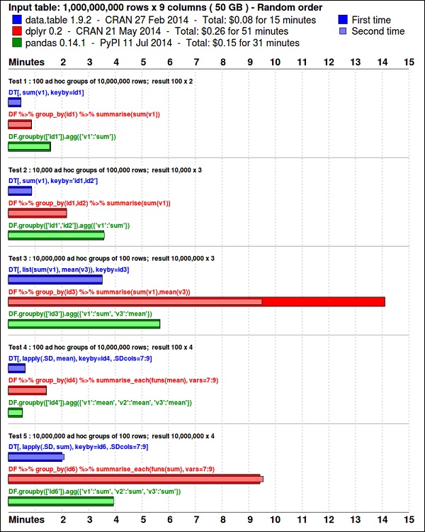
The ggplot2 package is great for data visualization. The data.table package is a great option to do fast and memory efficient summarization in R. A recent benchmark shows it is even faster than pandas, the python library used for similar tasks.
Take a look at the data using the following code. This code is also available in bda/part1/summarize_data/summarize_data.Rproj file.
library(nycflights13)
library(ggplot2)
library(data.table)
library(reshape2)

# Convert the flights data.frame to a data.table object and call it DT
DT <- as.data.table(flights)

# The data has 336776 rows and 16 columns
dim(DT)

# Take a look at the first rows
head(DT)

#   year    month  day   dep_time  dep_delay  arr_time  arr_delay  carrier
# 1: 2013     1     1      517       2         830         11       UA
# 2: 2013     1     1      533       4         850         20       UA
# 3: 2013     1     1      542       2         923         33       AA
# 4: 2013     1     1      544      -1        1004        -18       B6
# 5: 2013     1     1      554      -6         812        -25       DL
# 6: 2013     1     1      554      -4         740         12       UA

#     tailnum  flight  origin   dest    air_time   distance    hour   minute
# 1:  N14228   1545     EWR      IAH      227        1400       5       17
# 2:  N24211   1714     LGA      IAH      227        1416       5       33
# 3:  N619AA   1141     JFK      MIA      160        1089       5       42
# 4:  N804JB    725     JFK      BQN      183        1576       5       44
# 5:  N668DN    461     LGA      ATL      116        762        5       54
# 6:  N39463   1696     EWR      ORD      150        719        5       54
The following code has an example of data summarization.
### Data Summarization
# Compute the mean arrival delay
DT[, list(mean_arrival_delay = mean(arr_delay, na.rm = TRUE))]
#        mean_arrival_delay
# 1:           6.895377
# Now, we compute the same value but for each carrier
mean1 = DT[, list(mean_arrival_delay = mean(arr_delay, na.rm = TRUE)),
   by = carrier]
print(mean1)
#      carrier    mean_arrival_delay
# 1:      UA          3.5580111
# 2:      AA          0.3642909
# 3:      B6          9.4579733
# 4:      DL          1.6443409
# 5:      EV         15.7964311
# 6:      MQ         10.7747334
# 7:      US          2.1295951
# 8:      WN          9.6491199
# 9:      VX          1.7644644
# 10:     FL         20.1159055
# 11:     AS         -9.9308886
# 12:     9E          7.3796692
# 13:     F9         21.9207048
# 14:     HA         -6.9152047
# 15:     YV         15.5569853
# 16:     OO         11.9310345

# Now let’s compute to means in the same line of code
mean2 = DT[, list(mean_departure_delay = mean(dep_delay, na.rm = TRUE),
   mean_arrival_delay = mean(arr_delay, na.rm = TRUE)),
   by = carrier]
print(mean2)

#       carrier    mean_departure_delay   mean_arrival_delay
# 1:      UA            12.106073          3.5580111
# 2:      AA             8.586016          0.3642909
# 3:      B6            13.022522          9.4579733
# 4:      DL             9.264505          1.6443409
# 5:      EV            19.955390         15.7964311
# 6:      MQ            10.552041         10.7747334
# 7:      US             3.782418          2.1295951
# 8:      WN            17.711744          9.6491199
# 9:      VX            12.869421          1.7644644
# 10:     FL            18.726075         20.1159055
# 11:     AS             5.804775         -9.9308886
# 12:     9E            16.725769          7.3796692
# 13:     F9            20.215543         21.9207048
# 14:     HA             4.900585         -6.9152047
# 15:     YV            18.996330         15.5569853
# 16:     OO            12.586207         11.9310345

### Create a new variable called gain
# this is the difference between arrival delay and departure delay
DT[, gain:= arr_delay - dep_delay]

# Compute the median gain per carrier
median_gain = DT[, median(gain, na.rm = TRUE), by = carrier]
print(median_gain)
Big Data Analytics - Data Exploration
Exploratory data analysis is a concept developed by John Tuckey (1977) that consists on a new perspective of statistics. Tuckey’s idea was that in traditional statistics, the data was not being explored graphically, is was just being used to test hypotheses. The first attempt to develop a tool was done in Stanford, the project was called prim9. The tool was able to visualize data in nine dimensions, therefore it was able to provide a multivariate perspective of the data.
In recent days, exploratory data analysis is a must and has been included in the big data analytics life cycle. The ability to find insight and be able to communicate it effectively in an organization is fueled with strong EDA capabilities.
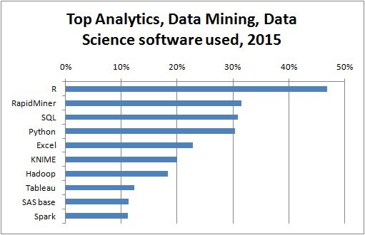
Based on Tuckey’s ideas, Bell Labs developed the S programming language in order to provide an interactive interface for doing statistics. The idea of S was to provide extensive graphical capabilities with an easy-to-use language. In today’s world, in the context of Big Data, R that is based on the S programming language is the most popular software for analytics.
The following program demonstrates the use of exploratory data analysis.
The following is an example of exploratory data analysis. This code is also available in part1/eda/exploratory_data_analysis.R file.
library(nycflights13)
library(ggplot2)
library(data.table)
library(reshape2)
# Using the code from the previous section
# This computes the mean arrival and departure delays by carrier.
DT <- as.data.table(flights)
mean2 = DT[, list(mean_departure_delay = mean(dep_delay, na.rm = TRUE),
mean_arrival_delay = mean(arr_delay, na.rm = TRUE)),
by = carrier]
# In order to plot data in R usign ggplot, it is normally needed to reshape the data
# We want to have the data in long format for plotting with ggplot
dt = melt(mean2, id.vars = ’carrier’)
# Take a look at the first rows
print(head(dt))
# Take a look at the help for ?geom_point and geom_line to find similar examples
# Here we take the carrier code as the x axis
# the value from the dt data.table goes in the y axis
# The variable column represents the color
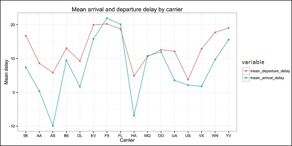
p = ggplot(dt, aes(x = carrier, y = value, color = variable, group = variable)) +
geom_point() + # Plots points
geom_line() + # Plots lines
theme_bw() + # Uses a white background
labs(list(title = 'Mean arrival and departure delay by carrier',
x = 'Carrier', y = 'Mean delay'))
print(p)
# Save the plot to disk
ggsave('mean_delay_by_carrier.png', p,
width = 10.4, height = 5.07)
The code should produce an image such as the following −