Machine Learning for Data Analysis

Machine learning is a subfield of computer science that deals with tasks such as pattern recognition, computer vision, speech recognition, text analytics and has a strong link with statistics and mathematical optimization. Applications include the development of search engines, spam filtering, Optical Character Recognition (OCR) among others. The boundaries between data mining, pattern recognition and the field of statistical learning are not clear and basically all refer to similar problems.

Machine learning can be divided in two types of task −

• Supervised Learning
• Unsupervised Learning

Supervised Learning

Supervised learning refers to a type of problem where there is an input data defined as a matrix X and we are interested in predicting a response y. Where X = {x₁, x₂, …, x_n} has n predictors and has two values y = {c₁, c₂}.

An example application would be to predict the probability of a web user to click on ads using demographic features as predictors. This is often called to predict the click through rate (CTR). Then y = {click, doesn’t − click} and the predictors could be the used IP address, the day he entered the site, the user’s city, country among other features that could be available.

Unsupervised Learning

Unsupervised learning deals with the problem of finding groups that are similar within each other without having a class to learn from. There are several approaches to the task of learning a mapping from predictors to finding groups that share similar instances in each group and are different with each other.

An example application of unsupervised learning is customer segmentation. For example, in the telecommunications industry a common task is to segment users according to the usage they give to the phone. This would allow the marketing department to target each group with a different product.

Big Data Analytics - Naive Bayes Classifier

Naive Bayes is a probabilistic technique for constructing classifiers. The characteristic assumption of the naive Bayes classifier is to consider that the value of a particular feature is independent of the value of any other feature, given the class variable.

Despite the oversimplified assumptions mentioned previously, naive Bayes classifiers have good results in complex real-world situations. An advantage of naive Bayes is that it only requires a small amount of training data to estimate the parameters necessary for classification and that the classifier can be trained incrementally.

Naive Bayes is a conditional probability model: given a problem instance to be classified, represented by a vector x = (x₁, …, x_n) representing some n features (independent variables), it assigns to this instance probabilities for each of K possible outcomes or classes.

p(Ck|x1,.....,xn)$$p(C_k|x_1,.....,x_n)$$

The problem with the above formulation is that if the number of features n is large or if a feature can take on a large number of values, then basing such a model on probability tables is infeasible. We therefore reformulate the model to make it simpler. Using Bayes theorem, the conditional probability can be decomposed as −

p(Ck|x)=p(Ck)p(x|Ck)p(x)$$p(C_k|x)=\frac{p(C_k)p(x|C_k)}{p(x)}$$

This means that under the above independence assumptions, the conditional distribution over the class variable C is −

p(Ck|x1,.....,xn)=1Zp(Ck)∏i=1np(xi|Ck)$$p(C_k|x_1,.....,x_n)=\frac{1}{Z}p(C_k)\prod _{i=1}^{n}p(x_i|C_k)$$

where the evidence Z = p(x) is a scaling factor dependent only on x₁, …, x_n, that is a constant if the values of the feature variables are known. One common rule is to pick the hypothesis that is most probable; this is known as the maximum a posteriori or MAP decision rule. The corresponding classifier, a Bayes classifier, is the function that assigns a class label y^=Ck$\hat{y}=C_k$ for some k as follows −

y^=argmaxp(Ck)∏i=1np(xi|Ck)$$\hat{y}=argmaxp(C_k)\prod _{i=1}^{n}p(x_i|C_k)$$

Implementing the algorithm in R is a straightforward process. The following example demonstrates how train a Naive Bayes classifier and use it for prediction in a spam filtering problem.

The following script is available in the bda/part3/naive_bayes/naive_bayes.R file.

# Install these packages 
pkgs = c("klaR", "caret", "ElemStatLearn") 
install.packages(pkgs)  
library('ElemStatLearn') 
library("klaR") 
library("caret")  

# Split the data in training and testing 
inx = sample(nrow(spam), round(nrow(spam) * 0.9)) 
train = spam[inx,] 
test = spam[-inx,]  

# Define a matrix with features, X_train 
# And a vector with class labels, y_train 
X_train = train[,-58] 
y_train = train$spam  
X_test = test[,-58] 
y_test = test$spam  
# Train the model 
nb_model = train(X_train, y_train, method = 'nb',  
   trControl = trainControl(method = 'cv', number = 3)) 

# Compute  
preds = predict(nb_model$finalModel, X_test)$class 
tbl = table(y_test, yhat = preds) 
sum(diag(tbl)) / sum(tbl) 
# 0.7217391 

As we can see from the result, the accuracy of the Naive Bayes model is 72%. This means the model correctly classifies 72% of the instances.

Big Data Analytics - K-Means Clustering

k-means clustering aims to partition n observations into k clusters in which each observation belongs to the cluster with the nearest mean, serving as a prototype of the cluster. This results in a partitioning of the data space into Voronoi cells.

Given a set of observations (x₁, x₂, …, x_n), where each observation is a d-dimensional real vector, k-means clustering aims to partition the n observations into k groups G = {G₁, G₂, …, G_k} so as to minimize the within-cluster sum of squares (WCSS) defined as follows −

argmin∑i=1k∑x∈Si∥x−μi∥2$$argmin\sum _{i=1}^k\sum _{x\in S_i}\parallel x-{\mu }_i{\parallel }^2$$

The later formula shows the objective function that is minimized in order to find the optimal prototypes in k-means clustering. The intuition of the formula is that we would like to find groups that are different with each other and each member of each group should be similar with the other members of each cluster.

The following example demonstrates how to run the k-means clustering algorithm in R.

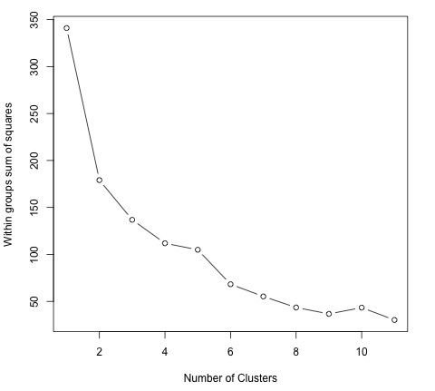
library(ggplot2)
# Prepare Data 
data = mtcars  

# We need to scale the data to have zero mean and unit variance 
data <- scale(data)  

# Determine number of clusters 
wss <- (nrow(data)-1)*sum(apply(data,2,var)) 
for (i in 2:dim(data)[2]) { 
   wss[i] <- sum(kmeans(data, centers = i)$withinss) 
}  

# Plot the clusters 
plot(1:dim(data)[2], wss, type = "b", xlab = "Number of Clusters", 
   ylab = "Within groups sum of squares")

In order to find a good value for K, we can plot the within groups sum of squares for different values of K. This metric normally decreases as more groups are added, we would like to find a point where the decrease in the within groups sum of squares starts decreasing slowly. In the plot, this value is best represented by K = 6.

Now that the value of K has been defined, it is needed to run the algorithm with that value.

# K-Means Cluster Analysis
fit <- kmeans(data, 5) # 5 cluster solution 

# get cluster means  
aggregate(data,by = list(fit$cluster),FUN = mean) 

# append cluster assignment 
data <- data.frame(data, fit$cluster) 

Big Data Analytics - Association Rules

Let I = i₁, i₂, ..., i_n be a set of n binary attributes called items. Let D = t₁, t₂, ..., t_m be a set of transactions called the database. Each transaction in D has a unique transaction ID and contains a subset of the items in I. A rule is defined as an implication of the form X ⇒ Y where X, Y ⊆ I and X ∩ Y = ∅.

The sets of items (for short item-sets) X and Y are called antecedent (left-hand-side or LHS) and consequent (right-hand-side or RHS) of the rule.

To illustrate the concepts, we use a small example from the supermarket domain. The set of items is I = {milk, bread, butter, beer} and a small database containing the items is shown in the following table.

Transaction ID	Items
1	milk, bread
2	bread, butter
3	beer
4	milk, bread, butter
5	bread, butter

An example rule for the supermarket could be {milk, bread} ⇒ {butter} meaning that if milk and bread is bought, customers also buy butter. To select interesting rules from the set of all possible rules, constraints on various measures of significance and interest can be used. The best-known constraints are minimum thresholds on support and confidence.

The support supp(X) of an item-set X is defined as the proportion of transactions in the data set which contain the item-set. In the example database in Table 1, the item-set {milk, bread} has a support of 2/5 = 0.4 since it occurs in 40% of all transactions (2 out of 5 transactions). Finding frequent item-sets can be seen as a simplification of the unsupervised learning problem.

The confidence of a rule is defined conf(X ⇒ Y ) = supp(X ∪ Y )/supp(X). For example, the rule {milk, bread} ⇒ {butter} has a confidence of 0.2/0.4 = 0.5 in the database in Table 1, which means that for 50% of the transactions containing milk and bread the rule is correct. Confidence can be interpreted as an estimate of the probability P(Y|X), the probability of finding the RHS of the rule in transactions under the condition that these transactions also contain the LHS.

In the script located in bda/part3/apriori.R the code to implement the apriori algorithm can be found.

# Load the library for doing association rules
# install.packages(’arules’) 
library(arules)  

# Data preprocessing 
data("AdultUCI") 
AdultUCI[1:2,]  
AdultUCI[["fnlwgt"]] <- NULL 
AdultUCI[["education-num"]] <- NULL  

AdultUCI[[ "age"]] <- ordered(cut(AdultUCI[[ "age"]], c(15,25,45,65,100)), 
   labels = c("Young", "Middle-aged", "Senior", "Old")) 
AdultUCI[[ "hours-per-week"]] <- ordered(cut(AdultUCI[[ "hours-per-week"]], 
   c(0,25,40,60,168)), labels = c("Part-time", "Full-time", "Over-time", "Workaholic")) 
AdultUCI[[ "capital-gain"]] <- ordered(cut(AdultUCI[[ "capital-gain"]], 
   c(-Inf,0,median(AdultUCI[[ "capital-gain"]][AdultUCI[[ "capitalgain"]]>0]),Inf)), 
   labels = c("None", "Low", "High")) 
AdultUCI[[ "capital-loss"]] <- ordered(cut(AdultUCI[[ "capital-loss"]], 
   c(-Inf,0, median(AdultUCI[[ "capital-loss"]][AdultUCI[[ "capitalloss"]]>0]),Inf)), 
   labels = c("none", "low", "high"))

In order to generate rules using the apriori algorithm, we need to create a transaction matrix. The following code shows how to do this in R.

# Convert the data into a transactions format
Adult <- as(AdultUCI, "transactions") 
Adult 
# transactions in sparse format with 
# 48842 transactions (rows) and 
# 115 items (columns)  

summary(Adult)  
# Plot frequent item-sets 
itemFrequencyPlot(Adult, support = 0.1, cex.names = 0.8)  

# generate rules 
min_support = 0.01 
confidence = 0.6 
rules <- apriori(Adult, parameter = list(support = min_support, confidence = confidence))

rules 
inspect(rules[100:110, ]) 
# lhs                             rhs                      support     confidence  lift
# {occupation = Farming-fishing} => {sex = Male}        0.02856148  0.9362416   1.4005486
# {occupation = Farming-fishing} => {race = White}      0.02831579  0.9281879   1.0855456
# {occupation = Farming-fishing} => {native-country     0.02671881  0.8758389   0.9759474
                                       = United-States} 

Big Data Analytics - Decision Trees

A Decision Tree is an algorithm used for supervised learning problems such as classification or regression. A decision tree or a classification tree is a tree in which each internal (nonleaf) node is labeled with an input feature. The arcs coming from a node labeled with a feature are labeled with each of the possible values of the feature. Each leaf of the tree is labeled with a class or a probability distribution over the classes.

A tree can be "learned" by splitting the source set into subsets based on an attribute value test. This process is repeated on each derived subset in a recursive manner called recursive partitioning. The recursion is completed when the subset at a node has all the same value of the target variable, or when splitting no longer adds value to the predictions. This process of top-down induction of decision trees is an example of a greedy algorithm, and it is the most common strategy for learning decision trees.

Decision trees used in data mining are of two main types −

• Classification tree − when the response is a nominal variable, for example if an email is spam or not.
• Regression tree − when the predicted outcome can be considered a real number (e.g. the salary of a worker).

Decision trees are a simple method, and as such has some problems. One of this issues is the high variance in the resulting models that decision trees produce. In order to alleviate this problem, ensemble methods of decision trees were developed. There are two groups of ensemble methods currently used extensively −

• Bagging decision trees − These trees are used to build multiple decision trees by repeatedly resampling training data with replacement, and voting the trees for a consensus prediction. This algorithm has been called random forest.
• Boosting decision trees − Gradient boosting combines weak learners; in this case, decision trees into a single strong learner, in an iterative fashion. It fits a weak tree to the data and iteratively keeps fitting weak learners in order to correct the error of the previous model.

# Install the party package
# install.packages('party') 
library(party) 
library(ggplot2)  

head(diamonds) 
# We will predict the cut of diamonds using the features available in the 
diamonds dataset. 
ct = ctree(cut ~ ., data = diamonds) 

# plot(ct, main="Conditional Inference Tree") 
# Example output 
# Response:  cut  
# Inputs:  carat, color, clarity, depth, table, price, x, y, z  

# Number of observations:  53940  
#  
# 1) table <= 57; criterion = 1, statistic = 10131.878 
#   2) depth <= 63; criterion = 1, statistic = 8377.279 
#     3) table <= 56.4; criterion = 1, statistic = 226.423 
#       4) z <= 2.64; criterion = 1, statistic = 70.393 
#         5) clarity <= VS1; criterion = 0.989, statistic = 10.48 
#           6) color <= E; criterion = 0.997, statistic = 12.829 
#             7)*  weights = 82  
#           6) color > E  

#Table of prediction errors 
table(predict(ct), diamonds$cut) 
#            Fair  Good Very Good Premium Ideal 
# Fair       1388   171        17       0    14 
# Good        102  2912       499      26    27 
# Very Good    54   998      3334     249   355 
# Premium      44   711      5054   11915  1167 
# Ideal        22   114      3178    1601 19988 
# Estimated class probabilities 
probs = predict(ct, newdata = diamonds, type = "prob") 
probs = do.call(rbind, probs) 
head(probs)

Big Data Analytics - Logistic Regression

Logistic regression is a classification model in which the response variable is categorical. It is an algorithm that comes from statistics and is used for supervised classification problems. In logistic regression we seek to find the vector β of parameters in the following equation that minimize the cost function.

logit(pi)=ln(pi1−pi)=β0+β1x1,i+...+βkxk,i$$logit(p_i)=ln\left(\frac{p_i}{1-p_i}\right)={\beta }_0+{\beta }_1{x}_{1,i}+...+{\beta }_k{x}_{k,i}$$

The following code demonstrates how to fit a logistic regression model in R. We will use here the spam dataset to demonstrate logistic regression, the same that was used for Naive Bayes.

From the predictions results in terms of accuracy, we find that the regression model achieves a 92.5% accuracy in the test set, compared to the 72% achieved by the Naive Bayes classifier.

library(ElemStatLearn)
head(spam) 

# Split dataset in training and testing 
inx = sample(nrow(spam), round(nrow(spam) * 0.8)) 
train = spam[inx,] 
test = spam[-inx,]  

# Fit regression model 
fit = glm(spam ~ ., data = train, family = binomial()) 
summary(fit)  

# Call: 
#   glm(formula = spam ~ ., family = binomial(), data = train) 
#  

# Deviance Residuals:  
#   Min       1Q   Median       3Q      Max   
# -4.5172  -0.2039   0.0000   0.1111   5.4944
# Coefficients: 
# Estimate Std. Error z value Pr(>|z|)     
# (Intercept) -1.511e+00  1.546e-01  -9.772  < 2e-16 *** 
# A.1         -4.546e-01  2.560e-01  -1.776 0.075720 .   
# A.2         -1.630e-01  7.731e-02  -2.108 0.035043 *   
# A.3          1.487e-01  1.261e-01   1.179 0.238591     
# A.4          2.055e+00  1.467e+00   1.401 0.161153     
# A.5          6.165e-01  1.191e-01   5.177 2.25e-07 *** 
# A.6          7.156e-01  2.768e-01   2.585 0.009747 **  
# A.7          2.606e+00  3.917e-01   6.652 2.88e-11 *** 
# A.8          6.750e-01  2.284e-01   2.955 0.003127 **  
# A.9          1.197e+00  3.362e-01   3.559 0.000373 *** 
# Signif. codes:  0 *** 0.001 ** 0.01 * 0.05 . 0.1  1  

### Make predictions 
preds = predict(fit, test, type = ’response’) 
preds = ifelse(preds > 0.5, 1, 0) 
tbl = table(target = test$spam, preds) 
tbl 

#         preds 
# target    0   1 
# email   535  23 
# spam     46 316 
sum(diag(tbl)) / sum(tbl) 
# 0.925

Big Data Analytics - Time Series Analysis

Time series is a sequence of observations of categorical or numeric variables indexed by a date, or timestamp. A clear example of time series data is the time series of a stock price. In the following table, we can see the basic structure of time series data. In this case the observations are recorded every hour.

Timestamp	Stock - Price
2015-10-11 09:00:00	100
2015-10-11 10:00:00	110
2015-10-11 11:00:00	105
2015-10-11 12:00:00	90
2015-10-11 13:00:00	120

Normally, the first step in time series analysis is to plot the series, this is normally done with a line chart.

The most common application of time series analysis is forecasting future values of a numeric value using the temporal structure of the data. This means, the available observations are used to predict values from the future.

The temporal ordering of the data, implies that traditional regression methods are not useful. In order to build robust forecast, we need models that take into account the temporal ordering of the data.

The most widely used model for Time Series Analysis is called Autoregressive Moving Average (ARMA). The model consists of two parts, an autoregressive (AR) part and a moving average (MA) part. The model is usually then referred to as the ARMA(p, q) model where p is the order of the autoregressive part and q is the order of the moving average part.

Autoregressive Model

The AR(p) is read as an autoregressive model of order p. Mathematically it is written as −

Xt=c+∑i=1PϕiXt−i+εt$$X_t=c+\sum _{i=1}^P{\varphi }_i{X}_{t-i}+{\epsilon }_t$$

where {φ₁, …, φ_p} are parameters to be estimated, c is a constant, and the random variable ε_t represents the white noise. Some constraints are necessary on the values of the parameters so that the model remains stationary.

Moving Average

The notation MA(q) refers to the moving average model of order q −

Xt=μ+εt+∑i=1qθiεt−i$$X_t=\mu +{\epsilon }_t+\sum _{i=1}^q{\theta }_i{\epsilon }_{t-i}$$

where the θ₁, ..., θ_q are the parameters of the model, μ is the expectation of X_t, and the ε_t, ε_{t − 1}, ... are, white noise error terms.

Autoregressive Moving Average

The ARMA(p, q) model combines p autoregressive terms and q moving-average terms. Mathematically the model is expressed with the following formula −

Xt=c+εt+∑i=1PϕiXt−1+∑i=1qθiεt−i$$X_t=c+{\epsilon }_t+\sum _{i=1}^P{\varphi }_i{X}_{t-1}+\sum _{i=1}^q{\theta }_i{\epsilon }_{t-i}$$

We can see that the ARMA(p, q) model is a combination of AR(p) and MA(q) models.

To give some intuition of the model consider that the AR part of the equation seeks to estimate parameters for X_{t − i} observations of in order to predict the value of the variable in X_t. It is in the end a weighted average of the past values. The MA section uses the same approach but with the error of previous observations, ε_{t − i}. So in the end, the result of the model is a weighted average.

The following code snippet demonstrates how to implement an ARMA(p, q) in R.

# install.packages("forecast")
library("forecast")  

# Read the data 
data = scan('fancy.dat') 
ts_data <- ts(data, frequency = 12, start = c(1987,1)) 
ts_data  
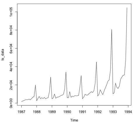
plot.ts(ts_data)

Plotting the data is normally the first step to find out if there is a temporal structure in the data. We can see from the plot that there are strong spikes at the end of each year.

The following code fits an ARMA model to the data. It runs several combinations of models and selects the one that has less error.

# Fit the ARMA model
fit = auto.arima(ts_data) 
summary(fit) 

# Series: ts_data  
# ARIMA(1,1,1)(0,1,1)[12]                     
#    Coefficients: 
#    ar1     ma1    sma1 
# 0.2401  -0.9013  0.7499 
# s.e.  0.1427   0.0709  0.1790 

#  
# sigma^2 estimated as 15464184:  log likelihood = -693.69 
# AIC = 1395.38   AICc = 1395.98   BIC = 1404.43 

# Training set error measures: 
#                 ME        RMSE      MAE        MPE        MAPE      MASE       ACF1 
# Training set   328.301  3615.374  2171.002  -2.481166  15.97302  0.4905797 -0.02521172

Big Data Analytics - Text Analytics

In this chapter, we will be using the data scraped in the part 1 of the book. The data has text that describes profiles of freelancers, and the hourly rate they are charging in USD. The idea of the following section is to fit a model that given the skills of a freelancer, we are able to predict its hourly salary.

The following code shows how to convert the raw text that in this case has skills of a user in a bag of words matrix. For this we use an R library called tm. This means that for each word in the corpus we create variable with the amount of occurrences of each variable.

library(tm)
library(data.table)  

source('text_analytics/text_analytics_functions.R') 
data = fread('text_analytics/data/profiles.txt') 
rate = as.numeric(data$rate) 
keep = !is.na(rate) 
rate = rate[keep]  

### Make bag of words of title and body 
X_all = bag_words(data$user_skills[keep]) 
X_all = removeSparseTerms(X_all, 0.999) 
X_all 

# <<DocumentTermMatrix (documents: 389, terms: 1422)>> 
#   Non-/sparse entries: 4057/549101 
# Sparsity           : 99% 
# Maximal term length: 80 
# Weighting          : term frequency - inverse document frequency (normalized) (tf-idf) 

### Make a sparse matrix with all the data 
X_all <- as_sparseMatrix(X_all)

Now that we have the text represented as a sparse matrix we can fit a model that will give a sparse solution. A good alternative for this case is using the LASSO (least absolute shrinkage and selection operator). This is a regression model that is able to select the most relevant features to predict the target.

train_inx = 1:200
X_train = X_all[train_inx, ] 
y_train = rate[train_inx]  
X_test = X_all[-train_inx, ] 
y_test = rate[-train_inx]  

# Train a regression model 
library(glmnet) 
fit <- cv.glmnet(x = X_train, y = y_train,  
   family = 'gaussian', alpha = 1,  
   nfolds = 3, type.measure = 'mae') 
plot(fit)  

# Make predictions 
predictions = predict(fit, newx = X_test) 
predictions = as.vector(predictions[,1]) 
head(predictions)  

# 36.23598 36.43046 51.69786 26.06811 35.13185 37.66367 
# We can compute the mean absolute error for the test data 
mean(abs(y_test - predictions)) 
# 15.02175

Now we have a model that given a set of skills is able to predict the hourly salary of a freelancer. If more data is collected, the performance of the model will improve, but the code to implement this pipeline would be the same.

Big Data Analytics - Online Learning

Online learning is a subfield of machine learning that allows to scale supervised learning models to massive datasets. The basic idea is that we don’t need to read all the data in memory to fit a model, we only need to read each instance at a time.

In this case, we will show how to implement an online learning algorithm using logistic regression. As in most of supervised learning algorithms, there is a cost function that is minimized. In logistic regression, the cost function is defined as −

J(θ)=−1m[∑i=1my(i)log(hθ(x(i)))+(1−y(i))log(1−hθ(x(i)))]$$J(\theta )=\frac{-1}{m}\left[\sum _{i=1}^m{y}^{(i)}log(h_{\theta }(x^{(i)}))+(1-y^{(i)})log(1-h_{\theta }(x^{(i)}))\right]$$

where J(θ) represents the cost function and h_θ(x) represents the hypothesis. In the case of logistic regression it is defined with the following formula −

hθ(x)=11+eθTx$$h_{\theta }(x)=\frac{1}{1+e^{{\theta }^{T}x}}$$

Now that we have defined the cost function we need to find an algorithm to minimize it. The simplest algorithm for achieving this is called stochastic gradient descent. The update rule of the algorithm for the weights of the logistic regression model is defined as −

θj:=θj−α(hθ(x)−y)x$${\theta }_j:={\theta }_j-\alpha (h_{\theta }(x)-y)x$$

There are several implementations of the following algorithm, but the one implemented in the vowpal wabbit library is by far the most developed one. The library allows training of large scale regression models and uses small amounts of RAM. In the creators own words it is described as: "The Vowpal Wabbit (VW) project is a fast out-of-core learning system sponsored by Microsoft Research and (previously) Yahoo! Research".

We will be working with the titanic dataset from a kaggle competition. The original data can be found in the bda/part3/vw folder. Here, we have two files −

• We have training data (train_titanic.csv), and
• unlabeled data in order to make new predictions (test_titanic.csv).

In order to convert the csv format to the vowpal wabbit input format use the csv_to_vowpal_wabbit.py python script. You will obviously need to have python installed for this. Navigate to the bda/part3/vw folder, open the terminal and execute the following command −

python csv_to_vowpal_wabbit.py

Note that for this section, if you are using windows you will need to install a Unix command line, enter the cygwin website for that.

Open the terminal and also in the folder bda/part3/vw and execute the following command −

vw train_titanic.vw -f model.vw --binary --passes 20 -c -q ff --sgd --l1 
0.00000001 --l2 0.0000001 --learning_rate 0.5 --loss_function logistic

Let us break down what each argument of the vw call means.

• -f model.vw − means that we are saving the model in the model.vw file for making predictions later
• --binary − Reports loss as binary classification with -1,1 labels
• --passes 20 − The data is used 20 times to learn the weights
• -c − create a cache file
• -q ff − Use quadratic features in the f namespace
• --sgd − use regular/classic/simple stochastic gradient descent update, i.e., nonadaptive, non-normalized, and non-invariant.
• --l1 --l2 − L1 and L2 norm regularization
• --learning_rate 0.5 − The learning rate αas defined in the update rule formula

The following code shows the results of running the regression model in the command line. In the results, we get the average log-loss and a small report of the algorithm performance.

-loss_function logistic
creating quadratic features for pairs: ff  
using l1 regularization = 1e-08 
using l2 regularization = 1e-07 

final_regressor = model.vw 
Num weight bits = 18 
learning rate = 0.5 
initial_t = 1 
power_t = 0.5 
decay_learning_rate = 1 
using cache_file = train_titanic.vw.cache 
ignoring text input in favor of cache input 
num sources = 1 

average    since         example   example  current  current  current 
loss       last          counter   weight    label   predict  features 
0.000000   0.000000          1      1.0    -1.0000   -1.0000       57 
0.500000   1.000000          2      2.0     1.0000   -1.0000       57 
0.250000   0.000000          4      4.0     1.0000    1.0000       57 
0.375000   0.500000          8      8.0    -1.0000   -1.0000       73 
0.625000   0.875000         16     16.0    -1.0000    1.0000       73 
0.468750   0.312500         32     32.0    -1.0000   -1.0000       57 
0.468750   0.468750         64     64.0    -1.0000    1.0000       43 
0.375000   0.281250        128    128.0     1.0000   -1.0000       43 
0.351562   0.328125        256    256.0     1.0000   -1.0000       43 
0.359375   0.367188        512    512.0    -1.0000    1.0000       57 
0.274336   0.274336       1024   1024.0    -1.0000   -1.0000       57 h 
0.281938   0.289474       2048   2048.0    -1.0000   -1.0000       43 h 
0.246696   0.211454       4096   4096.0    -1.0000   -1.0000       43 h 
0.218922   0.191209       8192   8192.0     1.0000    1.0000       43 h 

finished run 
number of examples per pass = 802 
passes used = 11 
weighted example sum = 8822 
weighted label sum = -2288 
average loss = 0.179775 h 
best constant = -0.530826 
best constant’s loss = 0.659128 
total feature number = 427878

Now we can use the model.vw we trained to generate predictions with new data.

vw -d test_titanic.vw -t -i model.vw -p predictions.txt 

The predictions generated in the previous command are not normalized to fit between the [0, 1] range. In order to do this, we use a sigmoid transformation.

# Read the predictions
preds = fread('vw/predictions.txt')  

# Define the sigmoid function 
sigmoid = function(x) { 
   1 / (1 + exp(-x)) 
} 
probs = sigmoid(preds[[1]])  

# Generate class labels 
preds = ifelse(probs > 0.5, 1, 0) 
head(preds) 
# [1] 0 1 0 0 1 0